17 Introduction to Vector Space
Thus far we have covered various forms of counting. But more advanced methods in NLP often rely on comparing instead. To understand these methods, we must get comfortable with the idea of vector space.
This chapter is a basic introduction to the concept of representing documents as vectors. We also introduce two basic vector-based measurement techniques: Euclidean distance and cosine similarity. A more advanced and in-depth guide to navigating vector space will be covered in Chapter 20.
A fictional example1: Daniel and Amos filled out a psychology questionnaire. The questionnaire measured three aspects of their personalities: extraversion, openness to experience, and neuroticism.
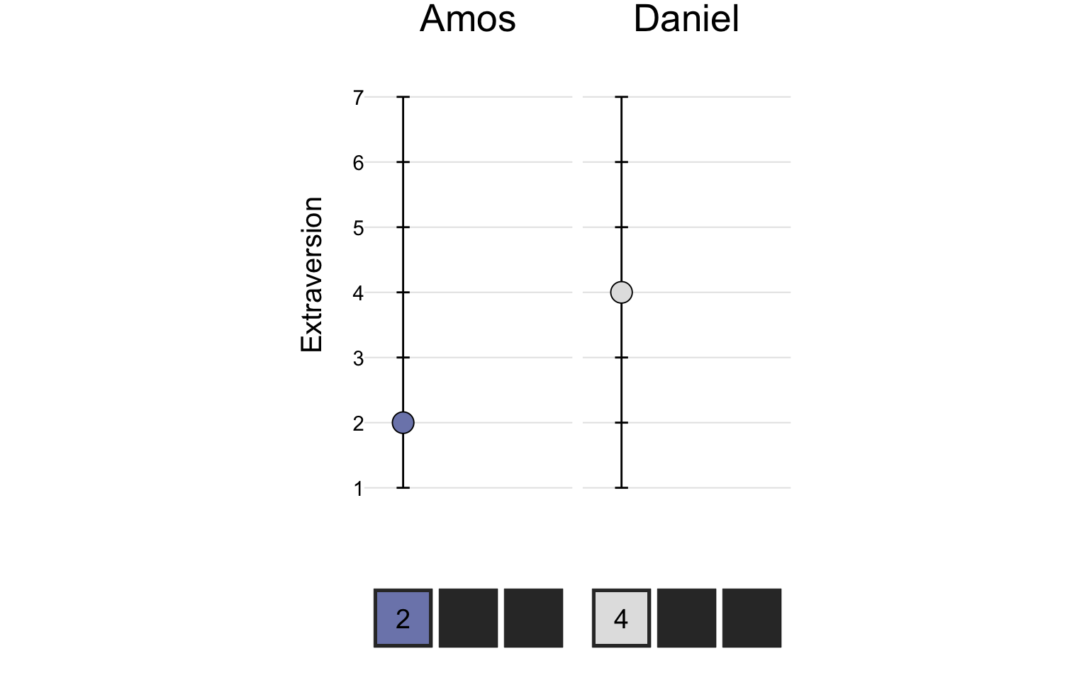
On the extraversion scale, Amos scored a 2 and Daniel scored a 4:
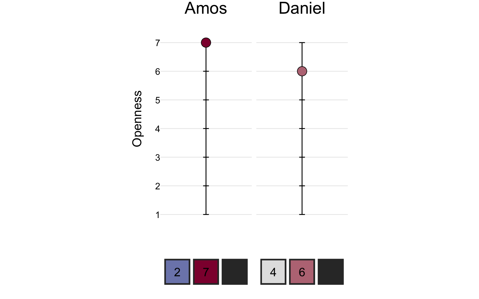
On the openness scale, Amos scored a 7 and Daniel scored a 6:
On the neuroticism scale, Amos scored a 3 and Daniel scored a 5.
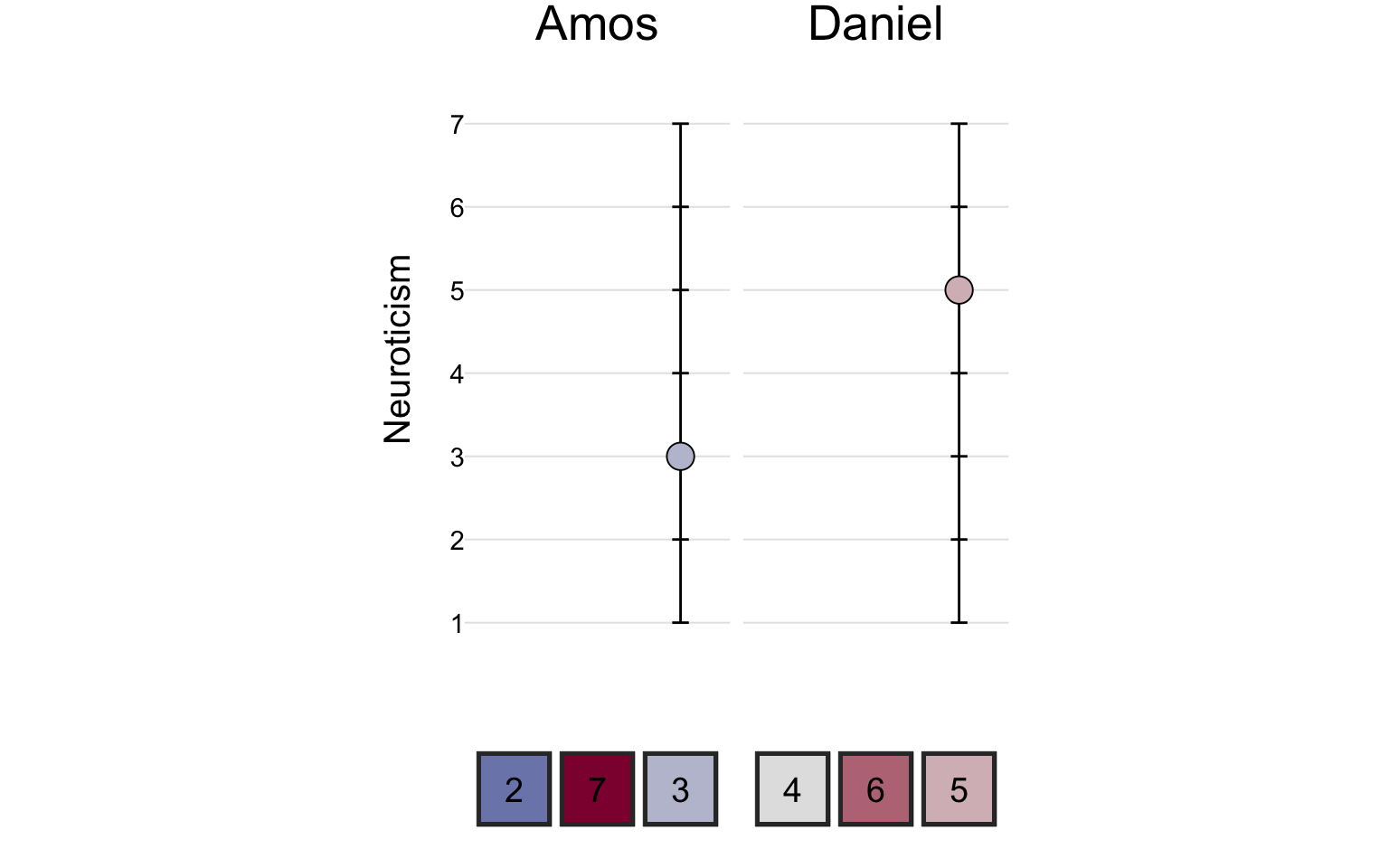
We can now represent each person’s personality as a list of three numbers, or a three dimensional vector. We can graph these vectors in three dimensional vector space:

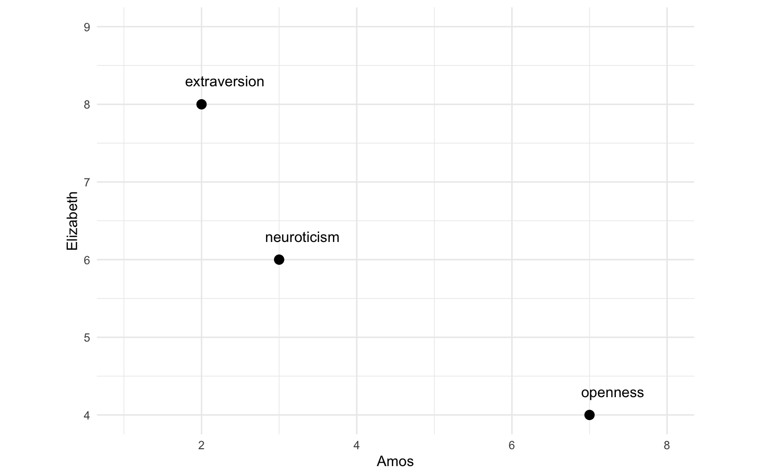
Now imagine that we encounter a third person, Elizabeth. We would like to know whether Elizabeth is more similar to Daniel or to Amos.
After graphing all three people in three-dimensional vector space, it becomes obvious that Elizabeth is more similar to Daniel than she is to Amos. Thinking of people (or any sort of observations) as vectors is powerful because it allows us to apply geometric reasoning to data. The beauty of this approach is that we can measure these things without knowing anything about what the dimensions represent. This will be important later.
Thus far we have discussed three-dimensional vector space. But what if we want to measure personality with the full Big-Five traits—openness, conscientiousness, extraversion, agreeableness, and neuroticism? Five dimensions would make it impossible to graph the data in an intuitive way as we have done above, but in a mathematical sense, it doesn’t matter. We can measure distance—and many other geometric concepts—just as easily in five-dimensional vector space as in three dimensions.
17.1 Distance and Similarity
When we added Elizabeth to the graph above, we could tell that she was more similar to Daniel than to Amos just by looking at the graph. But how do we quantify this similarity or difference?
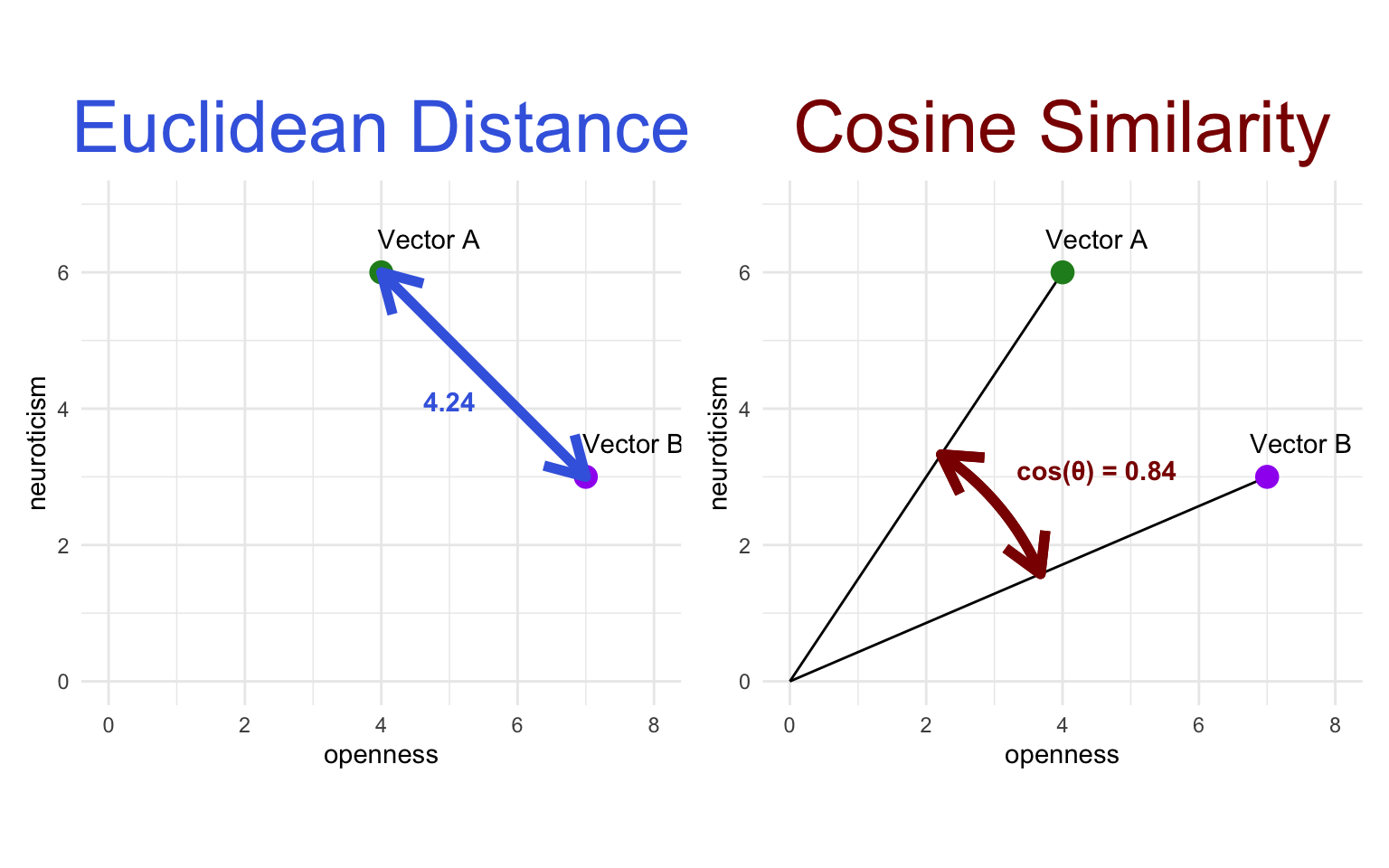
17.1.1 Euclidean Distance
The most straightforward way to measure the similarity between two points in space is to measure the distance between them. Euclidean distance is the simplest sort of distance—the length of the shortest straight line between the two points. The Euclidean distance between two vectors \(A\) and \(B\) can be calculated in any number of dimensions \(n\) using the following formula:
\[ d\left( A,B\right) = \sqrt {\sum _{i=1}^{n} \left( A_{i}-B_{i}\right)^2 } \]
A low Euclidean distance means two vectors are very similar. Let’s calculate the Euclidean distance between Daniel and Elizabeth, and between Amos and Elizabeth:
# dataset
personality
#> # A tibble: 3 × 4
#> person extraversion openness neuroticism
#> <chr> <dbl> <dbl> <dbl>
#> 1 Daniel 4 6 5
#> 2 Amos 2 7 3
#> 3 Elizabeth 8 4 6# Elizabeth's vector
eliza_vec <- personality |>
filter(person == "Elizabeth") |>
select(extraversion:neuroticism) |>
as.numeric()
# Euclidean distance function
euc_dist <- function(x, y){
diff <- x - y
sqrt(sum(diff^2))
}
# distance between Elizabeth and each person
personality_dist <- personality |>
rowwise() |>
mutate(
dist_from_eliza = euc_dist(c_across(extraversion:neuroticism), eliza_vec)
)
personality_dist#> # A tibble: 3 × 5
#> # Rowwise:
#> person extraversion openness neuroticism dist_from_eliza
#> <chr> <dbl> <dbl> <dbl> <dbl>
#> 1 Daniel 4 6 5 4.58
#> 2 Amos 2 7 3 7.35
#> 3 Elizabeth 8 4 6 0We now see that the closest person to Elizabeth is… Elizabeth herself, with a distance of 0. After that, the closest is Daniel. So we can conclude that Daniel has a more Elizabeth-like personality than Amos does.
17.1.2 Cosine Similarity
Besides Euclidean distance, the most common way to measure the similarity between two vectors is with cosine similarity. This is the cosine of the angle between the two vectors. Since the cosine of 0 is 1, a high cosine similarity (close to 1) means two vectors are very similar.
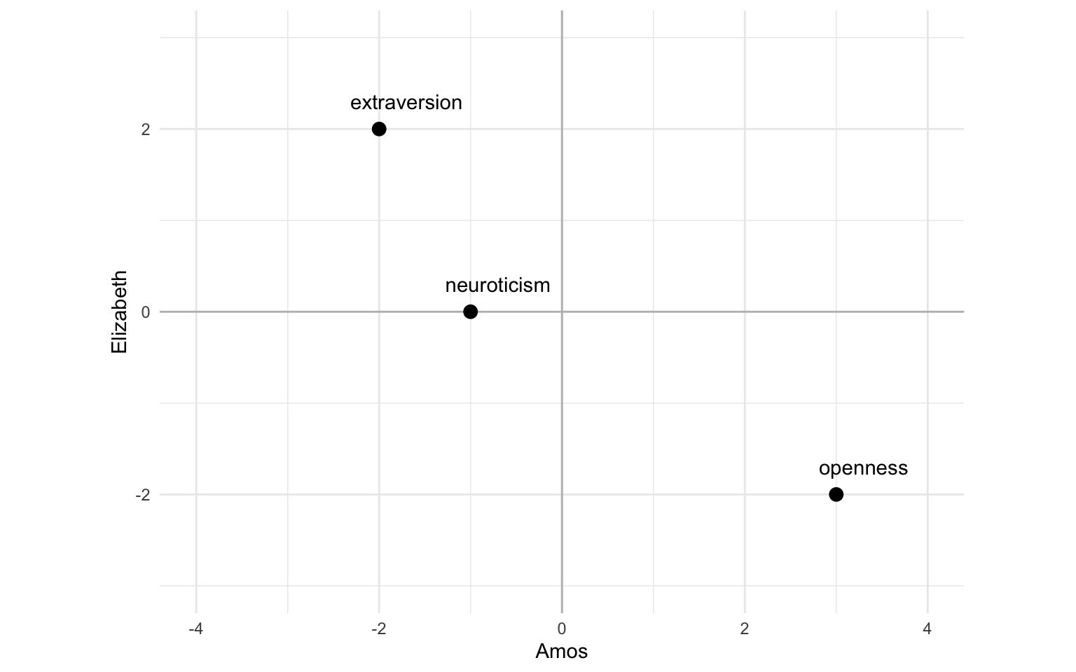
A nice thing about the cosine is that it is always between -1 and 1: When the two vectors are pointing in a similar direction, the cosine is close to 1, and when they are pointing in a near-opposite direction (180°), the cosine is close to -1.
Looking at the above visualization, you might wonder: Why should the angle be fixed at the zero point? What does the zero point have to do with anything? If you wondered this, good job. The reason: Cosine similarity works best when your vector space is centered at zero (or close to it). In other words, it works best when zero represents a medium level of each variable. This fact is sometimes taken for granted because, in practice, many vector spaces are already centered at zero. For example, word embeddings trained with word2vec, GloVe, and related models (Section 18.3) can be assumed to center at zero given sufficiently diverse training data because their training is based on the dot products between embeddings (the dot product is a close cousin of cosine similarity). The ubiquity of zero-centered vector spaces makes cosine similarity a very useful tool. Even so, not all vector spaces are zero-centered, so take a moment to consider the nature of your vector space before deciding which similarity or distance metric to use.
The formula for calculating cosine similarity might look a bit complicated:
\[ Cosine(A,B) = \frac{A \cdot B}{|A||B|} = \frac{\sum _{i=1}^{n} A_{i}B_{i}}{\sqrt {\sum _{i=1}^{n} A_{i}^2} \cdot \sqrt {\sum _{i=1}^{n} B_{i}^2}} \] In R though, it’s pretty simple. Let’s calculate the cosine similarity between Elizabeth and each of the other people in our sample. To make sure the vector space is centered at zero, we will subtract 4 from each value (the scales all range from 1 to 7).
# cosine similarity function
cos_sim <- function(x, y){
  dot <- x %*% y
  normx <- sqrt(sum(x^2))
  normy <- sqrt(sum(y^2))
  as.vector( dot / (normx*normy) )
}

# center at 0
eliza_vec_centered <- eliza_vec - 4
personality_sim <- personality |>
  mutate(across(extraversion:neuroticism, ~.x - 4))

# similarity between Elizabeth and each person
personality_sim <- personality_sim |>
  rowwise() |>
  mutate(
    similarity_to_eliza = cos_sim(c_across(extraversion:neuroticism), eliza_vec_centered)
  )

personality_sim
#> # A tibble: 3 × 5
#> # Rowwise:
#> person extraversion openness neuroticism similarity_to_eliza
#> <chr> <dbl> <dbl> <dbl> <dbl>
#> 1 Daniel 0 2 1 0.2
#> 2 Amos -2 3 -1 -0.598
#> 3 Elizabeth 4 0 2 1Once again, we see that the most similar person to Elizabeth is Elizabeth herself, with a cosine similarity of 1. The next closest, as before, is Daniel.
If you are comfortable with cosines, you might be happy with the explanation we have given so far. Nevertheless, it might be helpful to consider the relationship between cosine similarity and a more familiar statistic that ranges between -1 and 1: the Pearson correlation coefficient (i.e. regular old correlation). Cosine similarity measures the similarity between two vectors, while the correlation coefficient measures the similarity between two variables. Now just imagine our vectors as variables, with each dimension as an observation. Since we only compare two vectors at a time with cosine similarity, let’s start with Elizabeth and Amos:
Now imagine centering those variables at zero, like this:
When seen like this, the correlation is the same as the cosine similarity. In other words, the correlation between two vectors is the same as the cosine similarity between them when the values of each vector are centered at zero.2 Seeing cosine similarity as the non-centered version of correlation might give you extra intuition for why cosine similarity works best for vector spaces that are centered at zero.
17.2 The embedplyr Package
In the next few chapters, we will be performing lots more operations with vector embeddings. To streamline these operations and clarify the example code, we will use the embedplyr package, which is designed to make working with embeddings simple and fast.
# install embedplyr from Github
remotes::install_github("rimonim/embedplyr")A quick example: In Section 17.1.1, we used a custom function, euc_dist, along with rowwise() and c_across() to calculate the Euclidean distance between Elizabeth and each other person. With embedplyr we can do this much more simply using the get_sims() function:
# Elizabeth vector embedding
eliza_vec
#> [1] 8 4 6# distance between Elizabeth and each person
personality_dist <- personality |>
get_sims(
extraversion:neuroticism, # embedding columns
list(dist_from_eliza = eliza_vec), # scores to be calculated
method = "euclidean" # distance/similarity metric
)
personality_dist#> # A tibble: 3 × 2
#> person dist_from_eliza
#> <chr> <dbl>
#> 1 Daniel 4.58
#> 2 Amos 7.35
#> 3 Elizabeth 0We will introduce more embedplyr functions as they become relevant in the following chapters.
17.3 Word Counts as Vector Space
The advantage of thinking in vector space is that we can quantify similarities and differences even without understanding what any of the dimensions in the vector space are measuring. In the coming chapters, we will introduce methods that require this kind of relational thinking, since the dimensions of the vector space are abstract statistical contrivances. Even so, any collection of variables can be thought of as dimensions in a vector space. You might, for example, use distance or similarity metrics to analyze groups of word counts.
An example of word counts as relational vectors in research: Ireland & Pennebaker (2010) asked students to answer essay questions written in different styles. They then calculated dictionary-based word counts for both the questions and the answers using 9 linguistic word lists from LIWC (see Section 14.6), including personal pronouns (e.g. “I”, “you”), and articles (e.g, “a”, “the”). They treated these 9 word counts as a 9-dimensional vector for each text, and measured the similarity between questions and responses with a metric similar to Euclidean distance. They found that students automatically matched the linguistic style of the questions (i.e. answers were more similar to the question they were answering than to other questions) and that women and students with higher grades matched their answers especially closely to the style of the questions.
Alammar, J. (2019). The illustrated Word2vec. In Jay Alammar – Visualizing machine learning one concept at a time. http://jalammar.github.io/illustrated-word2vec/
Ireland, M. E., & Pennebaker, J. W. (2010). Language style matching in writing: Synchrony in essays, correspondence, and poetry. Journal of Personality and Social Psychology, 99(3), 549–571.
O’Connor, B. (2012). Cosine similarity, Pearson correlation, and OLS coefficients. In AI and Social Science. https://brenocon.com/blog/2012/03/cosine-similarity-pearson-correlation-and-ols-coefficients/